
library(sf)
library(rnaturalearth)

# Get low resolution Natural Earth data as map units instead of countries because of France
world <- ne_countries(scale = 110, type = "map_units")

# Save as geojson for Observable Plot
st_write(
  obj = world,
  dsn = "ne_110m_admin_0_countries.geojson",
  driver = "GeoJSON"
)

# Save medium resolution geojson
st_write(
  obj = ne_countries(scale = 50, type = "countries"),
  dsn = "ne_50m_admin_0_countries.geojson",
  driver = "GeoJSON"
)As part of Elon Musk’s weird Department of Government Efficiency’s unconstitutional rampage through the federal government, USAID’s ForeignAssistance.gov was taken offline on January 31, 2025. It reappeared on February 3, but it’s not clear how long it will be available, especially as USAID is gutted (despite court orders and injunctions to stop).
I study civil society, human rights, and foreign aid and rely on USAID aid data for several of my research projects, so as a backup, I used Datasette to create a mirror website/API of the entire ForeignAssistance.gov dataset at https://foreignassistance-data.andrewheiss.com/. Everything as of December 19, 2024 is available there, both as a queryable SQL database and as downloadable CSV files.
I also made a little frontend website with links to each individual dataset. As I built that website, I decided to try recreating the ForeignAssistance.gov dashboard, which had neat interactive maps and tables.

Since Quarto has native support for Observable JS for interactive work, and since I’ve meant to really dig into Observable and figure out how to make more interactive graphs, I figured I’d play around with the rescued USAID data.
So in this post, I show what I learned about working with geographic data and making pretty maps with Observable Plot,
WarningCaveat!
I’m really bad at Javascript! The code here is probably wildly inefficient and feels R-flavored.
But it works, and that’s all that matters :)
Working with map data
Get map data
Observable Plot uses the d3-geo module behind the scenes to parse and work with map data, and D3 typically works with data formatted as GeoJSON. There are tons of high quality geographic data sources online, like the US Census (they’ve been removing those in the past few weeks), IPUMS NHGIS, IPUMS IHGIS, and the Natural Earth project, and cities and states typically offer GIS data for public sector-related data. These data sources tend to be stored as shapefiles, which are a fairly complex (but standard) format for geographic data that involve multiple files.
Observable Plot/D3 might be able to work with shapefiles directly, but it’s nowhere in the documentation. They seem to expect GeoJSON instead. We could hunt around online for GeoJSON data, but—even better—we can use the {sf} package in R to convert any shapefile-based data into GeoJSON by setting driver = "GeoJSON" in sf::st_write(). Here we’ll load two datasets from Natural Earth—(1) small scale low resolution 1:110m data for mapping the whole world and (2) medium scale 1:50m data for mapping specific regions and countries—and convert them to GeoJSON files.
NoteMaybe skip intermediate saving?
We could probably use Quarto’s special R-to-OJS function ojs_define() and make these R objects directly accessible to OJS without needing to save intermediate files:
ojs_define(world = ne_countries(scale = 110, type = "map_units"))…but geographic data is complex and I don’t know how things like Observable Plot’s Plot.geo() handle data that’s not read as GeoJSON. So to keep things simple, I ended up just saving these as GeoJSON. 🤷♂️
Maps and projections with Observable Plot
We can load these into our document with OJS with FileAttachment():
world = FileAttachment("ne_110m_admin_0_countries.geojson").json()
world_medium = FileAttachment("ne_50m_admin_0_countries.geojson").json()
Check out the structure of world. It’s a FeatureCollection with a slot named crs with the projection information and a slot named features with entries for each country. Each country Feature has a slot named properties with columns like name, iso_a3, formal_en, pop_est, and other details.
worldTo plot it, we can use the Geo mark:
Plot.plot({
  marks: [
    Plot.geo(world)
  ]
})
To make things look nicer throughout this post, we’ll define some nicer colors for countries and land and ocean from CARTOColors:
carto_prism = [
  "#5F4690", "#1D6996", "#38A6A5", "#0F8554", "#73AF48", "#EDAD08",
  "#E17C05", "#CC503E", "#94346E", "#6F4070", "#994E95", "#666666"
]

// From R:
// clr_ocean <- colorspace::lighten("#88CCEE", 0.7)
clr_ocean = "#D9F0FF"

// From CARTOColors Peach 2
clr_land = "#facba6"
We’ll make the land be orange-ish, add some thin black borders around the countries, and include a blue background color with Plot.frame():
Plot.plot({
  marks: [
    Plot.frame({ fill: clr_ocean }),
    Plot.geo(world, {
      stroke: "black",
      strokeWidth: 0.5,
      fill: clr_land
    })
  ]
})
Built-in projections
Taking a round globe and smashing it on a two-dimensional surface always requires geometric shenanigans to get things flat. We can control how things get flattened by specifying the projection for the map. Here we’ll use the Equal Earth projection (invented in 2018 to show countries and continents at their true relative sizes to each other). Since projections contain relative height and width details, we need to specify a width for the plot now. I arbitrarily chose 1000 pixels here, which is the maximum width—it should autoshrink in smaller browser windows, and the height should be calculated automatically. Finally, instead of adding the background color with Plot.frame(), we can use Plot.sphere() to get a nicer background that uses the specified projection:
Plot.plot({
  projection: "equal-earth",
  width: 1000,
  marks: [
    Plot.sphere({ fill: clr_ocean }),
    Plot.geo(world, {
      stroke: "black",
      strokeWidth: 0.5,
      fill: clr_land
    })
  ]
})
The Observable Plot library includes a bunch of common built-in projections:
Other projections
Observable Plot can support any other D3 projection too. There are a whole bunch of projections in the main d3-geo module, and there’s a separate d3-geo-projection module for dozens of others. My favorite global projection is Robinson (the foundation for Equal Earth), which lives in d3-geo-projection. To use it, we can import the module with require() and then access it with d3_geo_projection.geoRobinson():
d3_geo_projection = require("d3-geo-projection")

Plot.plot({
  projection: d3_geo_projection.geoRobinson(),
  width: 1000,
  height: 500,
  marks: [
    Plot.sphere({ fill: clr_ocean }),
    Plot.geo(world, {
      stroke: "black",
      strokeWidth: 0.5,
      fill: clr_land
    })
  ]
})
Filtering map data and adjusting projections
Removing elements
Now that we have a nice projection, we can tweak the map a little. Antarctica is taking up a big proportion of the southern hemisphere, so we’ll filter it out. The world object that has all the map data keeps each country object inside a features slot:
world.featuresWe can filter it using Javascript’s .filter() function. To make sure that the resulting array keeps the geographic-ness of the data and is a FeatureCollection, we need to create a similarly structured object, with type and features slots:
world_sans_penguins = ({
  type: "FeatureCollection",
  features: world.features.filter(d => d.properties.iso_a3 !== "ATA")
})

Plot.plot({
  projection: d3_geo_projection.geoRobinson(),
  width: 1000,
  height: 500,
  marks: [
    Plot.sphere({ fill: clr_ocean }),
    Plot.geo(world_sans_penguins, {
      stroke: "black",
      strokeWidth: 0.5,
      fill: clr_land
    })
  ]
})
That works and Antarctica is gone, as expected, but in reality the map didn’t actually change that much. Even if we stop using the sphere background and just fill the plot frame, we can see that the area where Antarctica was is still there, it’s just missing the land itself:
Plot.plot({
  projection: d3_geo_projection.geoRobinson(),
  width: 1000,
  height: 500,
  marks: [
    Plot.frame({ fill: clr_ocean, stroke: "black", strokeWidth: 1 }),
    Plot.geo(world_sans_penguins, {
      stroke: "black",
      strokeWidth: 0.5,
      fill: clr_land
    })
  ]
})
Quick and dirty cheating method: change the width or height
One quick and dirty solution is to mess with the dimensions and shrink the height. After some trial and error, 430 pixels looks good:
Plot.plot({
  projection: d3_geo_projection.geoRobinson(),
  width: 1000,
  height: 430,
  marks: [
    Plot.frame({ fill: clr_ocean, stroke: "black", strokeWidth: 1 }),
    Plot.geo(world_sans_penguins, {
      stroke: "black",
      strokeWidth: 0.5,
      fill: clr_land
    })
  ]
})
While this works in this case, it’s not a universal solution. The only reason this works is because Antarctica happens to be at the bottom of the map. When you adjust the height of the plot area, the map itself is anchored to the top. Like, if we set the height to 215, we’ll get just the northern hemisphere:
Plot.plot({
  projection: d3_geo_projection.geoRobinson(),
  width: 1000,
  height: 215,
  marks: [
    Plot.frame({ fill: clr_ocean, stroke: "black", strokeWidth: 1 }),
    Plot.geo(world_sans_penguins, {
      stroke: "black",
      strokeWidth: 0.5,
      fill: clr_land
    })
  ]
})
As far as I can tell, there’s no way to anchor the map in any other position. If we filter the map data to only look at one continent, there’s no easy way to focus on just that continent by adjusting only the width or height options. Here’s Africa all by itself in a big empty plot area:
just_africa = ({
    type: "FeatureCollection",
    features: world.features.filter(d => d.properties.continent == "Africa")
})

Plot.plot({
  projection: d3_geo_projection.geoRobinson(),
  width: 1000,
  height: 430,
  marks: [
    Plot.frame({ fill: clr_ocean, stroke: "black", strokeWidth: 1 }),
    Plot.geo(just_africa, {
      stroke: "black",
      strokeWidth: 0.5,
      fill: clr_land
    })
  ]
})
If we adjust the width or the height, the plot area will be resized with the map anchored in the top left corner so we’re left with just the northwestern part of Africa (and big empty areas where North America, South America, and Europe would be):
Plot.plot({
  projection: d3_geo_projection.geoRobinson(),
  width: 550,
  height: 215,
  marks: [
    Plot.frame({ fill: clr_ocean, stroke: "black", strokeWidth: 1 }),
    Plot.geo(just_africa, {
      stroke: "black",
      strokeWidth: 0.5,
      fill: clr_land
    })
  ]
})
That’s not great, but there are better ways!
Built-in projections and domain settings
The official Observable Plot method for fitting the plot window to a specific area of the map is to define a “domain” for one of the built-in projections to zoom in on specific areas. The documentation shows how to use special functions in d3-geo to create a circle around a point, but you can also pass a GeoJSON object and Plot will use its boundaries for the domain. The built-in projection options also let us control the outside margin of the domain with inset.
Here’s the world map without Antarctica with the Equal Earth projection, with the projection resized to fit within the bounds of world_sans_penguins, with 10 pixels of padding around the landmass. Antarctica is gone now and the rest of the map is vertically centered within the plot area:
Plot.plot({
  projection: {
    type: "equal-earth",
    domain: world_sans_penguins,
    inset: 10
  },
  width: 1000,
  marks: [
    Plot.frame({ fill: clr_ocean, stroke: "black", strokeWidth: 1 }),
    Plot.geo(world_sans_penguins, {
      stroke: "black",
      strokeWidth: 0.5,
      fill: clr_land
    })
  ]
})
We can see what’s happening behind the scenes if we add Plot.sphere() back in. The rounded globe area is still there, but it’s shifted down and out of the frame. We’re essentially panning around and zooming in on the Equal Earth projection:
Plot.plot({
  projection: {
    type: "equal-earth",
    domain: world_sans_penguins,
    inset: 10
  },
  width: 1000,
  marks: [
    Plot.frame({ stroke: "black", strokeWidth: 1 }),
    Plot.sphere({ fill: clr_ocean }),
    Plot.geo(world_sans_penguins, {
      stroke: "black",
      strokeWidth: 0.5,
      fill: clr_land
    })
  ]
})
Passing a GeoJSON object as the domain is really neat because it makes it straightforward to zoom in on specific areas. For instance, here’s the complete medium resolution world map zoomed in around the just_africa object, which keeps non-African countries in the Middle East and southern Europe:
Plot.plot({
  projection: {
    type: "equal-earth",
    domain: just_africa,
    inset: 10
  },
  width: 600,
  height: 600,
  marks: [
    Plot.frame({ fill: clr_ocean, stroke: "black", strokeWidth: 1 }),
    Plot.geo(world_medium, {
      stroke: "black",
      strokeWidth: 0.5,
      fill: clr_land
    })
  ]
})
We could also extract Africa from the medium resolution world map and plot only that continent, omitting the Middle East and Europe:
just_africa_medium = ({
    type: "FeatureCollection",
    features: world_medium.features.filter(d => d.properties.continent == "Africa")
})

Plot.plot({
  projection: {
    type: "equal-earth",
    domain: just_africa,
    inset: 10
  },
  width: 600,
  height: 600,
  marks: [
    // Use a white background since we don't want to make it look like
    // the Sinai peninsula has a coastline
    Plot.frame({ fill: "white", stroke: "black", strokeWidth: 1 }),
    Plot.geo(just_africa_medium, {
      stroke: "black",
      strokeWidth: 0.5,
      fill: clr_land
    })
  ]
})
Other projections and .fitExtent()
Unfortunately, it’s a little bit trickier to set the domain and inset for projections that aren’t built in to Plot. We can’t do this:
Plot.plot({
  projection: {
    type: d3_geo_projection.geoRobinson(),
    domain: world_sans_penguins,
    inset: 10
  },
  ...
})
Instead, we need to adjust the size of the projection window itself and build in the inset with d3-geo’s .fitExtent(). This function takes four arguments in an array like [[x1, y1], [x2, y2]], defining the top left and bottom right corners (in pixels) of a window that is centered in the middle of a given GeoJSON object. Here, for instance, we create a copy of the Robinson projection that has a window around just_africa with a top left corner at (30, 30) and a bottom right corner at (570, 570):
inset_africa = 30
africa_map_width = 600
africa_map_height = 600

africa_robinson = d3_geo_projection.geoRobinson()
  .fitExtent(
    [[inset_africa, inset_africa],  // Top left
     [africa_map_width - inset_africa, africa_map_height - inset_africa]],  // Bottom right
    just_africa
  )

Plot.plot({
  projection: africa_robinson,
  width: africa_map_width,
  height: africa_map_height,
  marks: [
    Plot.frame({ fill: clr_ocean, stroke: "black", strokeWidth: 1 }),
    Plot.geo(world_sans_penguins, {
      stroke: "black",
      strokeWidth: 0.5,
      fill: clr_land
    })
  ]
})
We can use the same approach with individual countries. For extra fun, we’ll fill these countries with distinct colors using Natural Earth’s mapcolor7 column, which assigns countries one of 7 different colors that don’t border other countries (so neighboring countries will never be the same color). We’ll also add some labels in the middle of each country.
egypt = world_medium.features.find(d => d.properties.name === "Egypt")

inset_egypt = 75
egypt_map_width = 600
egypt_map_height = 600

robinson_egypt = d3_geo_projection.geoRobinson()
  .fitExtent(
    [[inset_egypt, inset_egypt],  // Top left
     [egypt_map_width - inset_egypt, egypt_map_height - inset_egypt]],  // Bottom right
    egypt
  )

Plot.plot({
  projection: robinson_egypt,
  width: egypt_map_width,
  height: egypt_map_height,
  marks: [
    Plot.frame({ fill: clr_ocean, stroke: "black", strokeWidth: 1 }),
    Plot.geo(world_medium, Plot.centroid({
      fill: d => d.properties.mapcolor7,
      stroke: "black",
      strokeWidth: 0.5
    })),
    Plot.geo(egypt, { stroke: "yellow", strokeWidth: 3 }),
    Plot.tip(world_medium.features, Plot.centroid({
      title: d => d.properties.name,
      anchor: "top",
      fontSize: 13,
      fontWeight: "bold",
      textPadding: 3
    }))
  ],
  color: {
    range: carto_prism
  }
})
The approach works for the whole world_sans_penguins object as well. This addresses our original problem—here’s a world map with the Robinson projection without Antarctica that fills the plot area correctly:
inset_world = 10
world_map_width = 1000
world_map_height = 450

world_sans_penguins_robinson = d3_geo_projection.geoRobinson()
  .fitExtent(
    [[inset_world, inset_world],
     [world_map_width - inset_world, world_map_height - inset_world]],
    world_sans_penguins
  )

Plot.plot({
  projection: world_sans_penguins_robinson,
  width: world_map_width,
  height: world_map_height,
  marks: [
    Plot.frame({ fill: clr_ocean, stroke: "black", strokeWidth: 1 }),
    Plot.geo(world_sans_penguins, {
      stroke: "black",
      strokeWidth: 0.5,
      fill: clr_land
    })
  ]
})
Arbitrary areas and .fitExtent()
For bonus fun, this approach also works for any arbitrary rectangles. For example, we can use OpenStreetMap’s neat Export tool to pick the top, bottom, left, and right edges of a box that focuses on Western Europe.
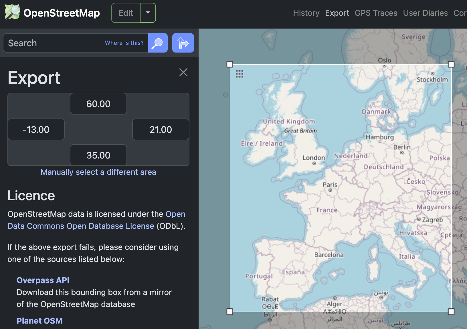
We can then use those coordinates to create a MultiPoint geometric feature/object, which essentially acts like a rectangular fake country/region that can be used as the domain or extent of the map:
inset_europe = 10
europe_map_width = 800
europe_map_height = 800

europe_box = ({
  type: "Feature",
  geometry: {
    type: "MultiPoint",
    coordinates: [
      [-13, 35],  // [left/west, bottom/south] (or bottom left corner)
      [21, 60]    // [right/east, top/north]   (or top right corner)
    ]
  }
})

europe_robinson = d3_geo_projection.geoRobinson()
  .fitExtent(
    [[inset_europe, inset_europe],
     [europe_map_width - inset_europe, europe_map_height - inset_europe]],
    europe_box
  )

Plot.plot({
  projection: europe_robinson,
  width: europe_map_width,
  height: europe_map_height,
  marks: [
    Plot.frame({ fill: clr_ocean, stroke: "black", strokeWidth: 1 }),
    Plot.geo(world_medium, Plot.centroid({
      fill: d => d.properties.mapcolor9,
      stroke: "white",
      strokeWidth: 0.25
    })),
    Plot.tip(world.features, Plot.centroid({
      title: d => d.properties.name,
      anchor: "bottom",
      fontSize: 13,
      fontWeight: "bold",
      textPadding: 3
    }))
  ],
  color: {
    range: carto_prism
  }
})
Working with USAID data
Get USAID data
To make it easier to access and filter and manipulate things, I put the rescued data on a Datasette instance, which is nice front-end for an SQLite database. This makes it possible to run SQL queries directly in the browser and generate custom datasets without needing to load the full massive CSV files into R or Python or Stata or whatever.
For example, one of the rescued USAID datasets is named us_foreign_aid_country and it contains 22,000+ rows, with data on aid obligations, appropriations, and disbursements starting in 1999.
If we want to get a total of all constant USD aid obligations by country in 2023, omitting regional and world totals, we could do something like this with R and {dplyr}:
library(tidyverse)

# Download the raw CSV and put it somewhere
us_foreign_aid_country <- read_csv("us_foreign_aid_country.csv")

us_foreign_aid_country |>
  filter(
    `Fiscal Year` == 2023,
    `Transaction Type Name` == "Obligations",
    !str_detect(`Country Name`, "Region"),
    `Country Name` != "World"
  ) |>
  group_by(`Country Code`, `Country Name`, `Region Name`) |>
  summarize(total_constant_amount = sum(constant_amount)) |>
  arrange(desc(total_constant_amount))
#>  A tibble: 176 × 4
#>  Groups:   Country Code, Country Name [176]
#>   `Country Code` `Country Name`   `Region Name`                total_constant_amount
#>   <chr>          <chr>            <chr>                                        <dbl>
#> 1 UKR            Ukraine          Europe and Eurasia                     17193710403
#> 2 ISR            Israel           Middle East and North Africa            3302860882
#> 3 JOR            Jordan           Middle East and North Africa            1686862605
#> 4 EGY            Egypt            Middle East and North Africa            1503609426
#> 5 ETH            Ethiopia         Sub-Saharan Africa                      1457374911
#> 6 SOM            Somalia          Sub-Saharan Africa                      1181033990
#> 7 NGA            Nigeria          Sub-Saharan Africa                      1019947490
#> 8 COD            Congo (Kinshasa) Sub-Saharan Africa                       990456757
#> 9 AFG            Afghanistan      South and Central Asia                   886536741
#> 0 KEN            Kenya            Sub-Saharan Africa                       846303488
#>  ℹ 166 more rows
#>  ℹ Use `print(n = ...)` to see more rows
Or we could get that data extract directly from the database without needing to load the huge original CSV file. We can run an SQL query like this at the Datasette website:
SELECT "Country Code", "Country Name", "Region Name", SUM("constant_amount") AS total_constant_amount
  FROM "./us_foreign_aid_country"
  WHERE
    "Fiscal Year" = '2023'
    AND "Transaction Type Name" = 'Obligations'
    AND "Country Name" NOT LIKE '%Region%'
    AND "Country Name" != "World"
  GROUP BY "Country Code", "Country Name", "Region Name"
  ORDER BY total_constant_amount DESC;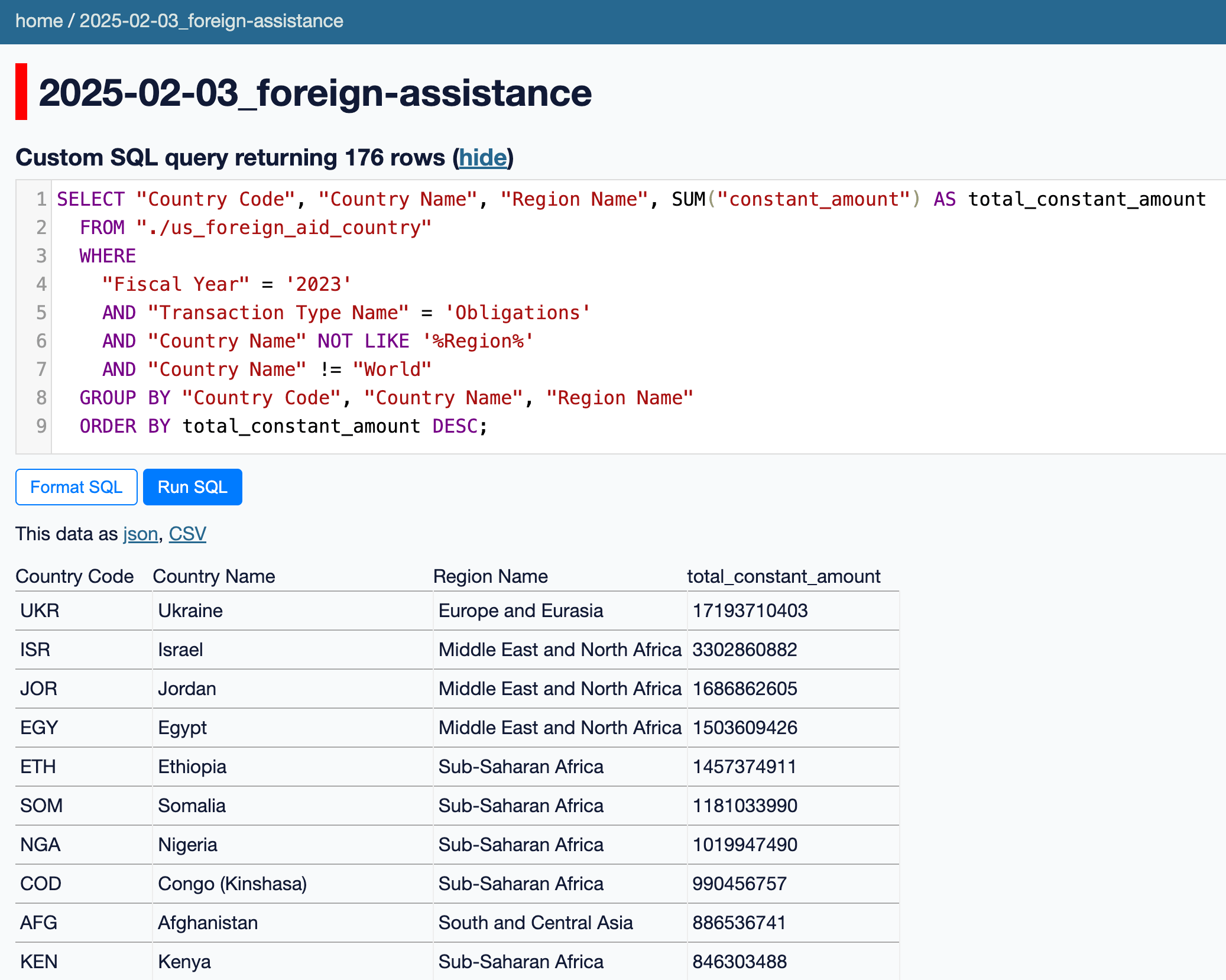
Since we’re working with interactive Observable Javascript, we can load that data directly into the browser instead of downloading intermediate CSV files. There’s a neat Datasette database client for Observable that lets us run SQL queries (there are lots of other clients too, if you want to connect to things like DuckDB, SQLite, MySQL, Snowflake, and so on).
import { DatasetteClient } from "@ambassadors/datasette-client"

aid_db = new DatasetteClient(
  "https://foreignassistance-data.andrewheiss.com/2025-02-03_foreign-assistance"
)

recipient_countries = await aid_db.sql`
  SELECT "Country Code", "Country Name", "Region Name", SUM("constant_amount") AS total_constant_amount
  FROM "./us_foreign_aid_country"
  WHERE
    "Fiscal Year" = '2023'
    AND "Transaction Type Name" = 'Obligations'
    AND "Country Name" NOT LIKE '%Region%'
    AND "Country Name" != "World"
  GROUP BY "Country Code", "Country Name", "Region Name"
  ORDER BY total_constant_amount DESC;
`
Through the magic of this Datasette client, we now have a pre-summarized dataset to work with!
recipient_countriesConnect USAID data to the map data
Following Observable Plot’s choropleth tutorial, to show these totals on a map, we need to create a Map object,1 which is like a Python dictionary or an R data frame with two columns, where we have (1) a name that shares a name with something in the geographic data, like an ISO3 country code, and (2) a value with the thing we want to plot.
1 This term is admittedly confusing because it has nothing to do with geographic maps and is instead related to functional programming.
country_totals = new Map(recipient_countries.map(d => [d["Country Code"], d.total_constant_amount]))
country_totals
This lets us get specific totals with the .get() method. Here’s Ukraine, for example:
country_totals.get("UKR")We can feed the ISO3 code of each country-level geographic shape into this country_totals object to extract the total amount of aid for each country. We’ll use the Antarctica-free Robinson projection we made earlier, and we’ll remove the ocean fill since we’ll ultimately make this interactive and hoverable:
Plot.plot({
  projection: world_sans_penguins_robinson,
  width: world_map_width,
  height: world_map_height,
  marks: [
    Plot.frame({ stroke: "black", strokeWidth: 1} ),
    Plot.geo(world_sans_penguins, Plot.centroid({
      fill: d => country_totals.get(d.properties.iso_a3)
    }))
  ]
})
Improving the map
We have a choropleth! But this is hardly publication worthy. We need to fix a bunch of issues with it.
First, countries that don’t receive aid don’t appear in the map. Let’s add borders to all the countries:
Plot.plot({
  projection: world_sans_penguins_robinson,
  width: world_map_width,
  height: world_map_height,
  marks: [
    Plot.frame({ stroke: "black", strokeWidth: 1} ),
    Plot.geo(world_sans_penguins, Plot.centroid({
      fill: d => country_totals.get(d.properties.iso_a3)
    })),
    Plot.geo(world_sans_penguins, {
      stroke: "black",
      strokeWidth: 0.5
    })
  ]
})
The coloring here is gross because of some huge outliers (Ukraine) that make most countries black/dark blue. There’s also no legend to show what these values are. We can address all of this by adjusting the legend options. We’ll log total aid, include the legend, add a nice label, and use a single-hue coloring scheme with gray for countries without aid:
Plot.plot({
  projection: world_sans_penguins_robinson,
  width: world_map_width,
  height: world_map_height,
  marks: [
    Plot.frame({ stroke: "black", strokeWidth: 1} ),
    Plot.geo(world_sans_penguins, Plot.centroid({
      fill: d => country_totals.get(d.properties.iso_a3)
    })),
    Plot.geo(world_sans_penguins, {
      stroke: "black",
      strokeWidth: 0.5
    })
  ],
  color: {
    scheme: "blues",
    unknown: "#f2f2f2",
    type: "log",
    legend: true,
    label: "Total obligations",
  }
})
Next, let’s make this interactive by turning on hovering tooltips:
Plot.plot({
  projection: world_sans_penguins_robinson,
  width: world_map_width,
  height: world_map_height,
  marks: [
    Plot.frame({ stroke: "black", strokeWidth: 1} ),
    Plot.geo(world_sans_penguins, Plot.centroid({
      fill: d => country_totals.get(d.properties.iso_a3),
      tip: true
    })),
    Plot.geo(world_sans_penguins, {
      stroke: "black",
      strokeWidth: 0.5
    })
  ],
  color: {
    scheme: "blues",
    unknown: "#f2f2f2",
    type: "log",
    legend: true,
    label: "Total obligations",
  }
})
That’s so cool. Hover over Mexico and you’ll see “Total obligations 232,214,023”.
We can make this tooltip more informative by including the country name and formatting the amount to show dollars. Instead of using tip: true, we can add the country name as a channel (Observable Plot’s version of a ggplot aesthetic), and format the tip so that the country name comes first and the total amount is formatted with d3.format():
Plot.plot({
  projection: world_sans_penguins_robinson,
  width: world_map_width,
  height: world_map_height,
  marks: [
    Plot.frame({ stroke: "black", strokeWidth: 1} ),
    Plot.geo(world_sans_penguins, Plot.centroid({
      fill: d => country_totals.get(d.properties.iso_a3),
      channels: {
        Country: d => d.properties.name,
      },
      tip: {
        format: {
          Country: true,
          fill: d3.format("$,d")
        }
      }
    })),
    Plot.geo(world_sans_penguins, {
      stroke: "black",
      strokeWidth: 0.5
    })
  ],
  color: {
    scheme: "blues",
    unknown: "#f2f2f2",
    type: "log",
    legend: true,
    label: "Total obligations",
  }
})
Now hover over Mexico and you’ll see the country name and the amount of aid in dollars.
Fixing labelling issues
We have two final super minor issues to address.
First hover over a country that didn’t receive aid, like the United States or Australia. The total reported aid displays as “$NaN”. That’s gross. It’d be nicer if it said something else, like “$0” or “No aid” or something more informative.
To fix this, we can make a little function that formats the given value as a dollar amount if it’s an actual value, and formats it as something else if it’s missing or not a number (like log(0)):
function format_aid_total(value) {
  return value ? d3.format("$,d")(value) : "No aid";
}
That works nicely:
format_aid_total(394023)format_aid_total(NaN)The other problem is in the legend, which uses a logarithmic scale and includes breaks for 10k, 1M, 100M, and 10G, representing $10,000, $1 million, $100 million, and $10 billion in aid.
The issue is the $10 billion, which is abbreviated with “G”.
This is happening because d3.format() uses SI (Système international d’unités, or International System of Units) values for its numeric formats, which means that it uses SI metric prefixes. Those legend breaks, therefore, actually technically mean this:
- 10k: 10 kilodollars
- 1M: 1 megadollar
- 100M: 100 megadollars
- 10G: 10 gigadollars
lol, I should start talking about big dollar amounts with these values (“the 2022 US federal budget deficit was 1.4 teradollars”)
The first letters of many of these SI prefixes happen to line up with US-style large numbers:
- In the US we already commonly use “k” for thousand
- The initial “m” in “mega” aligns with “million”
- The initial “t” in tera aligns with “trillion”
But “giga” doesn’t align with “billion”, hence the strange “G” here for dollar amounts.
People have requested that d3-format include an option for switching the abbreviation from G to B, but the developers haven’t added it (and probably won’t). Instead, a common recommended fix is to replace all “G”s with “B”s:
number_in_billions = 13840918291  // A big number I randomly typed

// Billions of dollars instead of SI-style gigadollars
d3.format("$.4s")(number_in_billions).replace("G", "B")
We can add format_aid_total() and the .replace("G", "B") tweak and fix the labels in our interactive map:
Plot.plot({
  projection: world_sans_penguins_robinson,
  width: world_map_width,
  height: world_map_height,
  marks: [
    Plot.frame({ stroke: "black", strokeWidth: 1} ),
    Plot.geo(world_sans_penguins, Plot.centroid({
      fill: d => country_totals.get(d.properties.iso_a3),
      channels: {
        Country: d => d.properties.name,
      },
      tip: {
        format: {
          Country: true,
          fill: d => format_aid_total(d)
        }
      }
    })),
    Plot.geo(world_sans_penguins, {
      stroke: "black",
      strokeWidth: 0.5
    })
  ],
  color: {
    scheme: "blues",
    unknown: "#f2f2f2",
    type: "log",
    legend: true,
    label: "Total obligations",
    tickFormat: d => d3.format("$0.2s")(d).replace("G", "B")
  }
})
Some final tweaks
We’re so close! Just a couple final incredibly minor changes:
- We’ll boost the font size of the tooltip a little and increase the font size of the legend
- We’ll switch from the built-in ColorBrewer
bluespalette to show how to use custom gradients, like CARTOColors’s PurpOr sequential palette
Plot.plot({
  projection: world_sans_penguins_robinson,
  width: world_map_width,
  height: world_map_height,
  marks: [
    Plot.frame({ stroke: "black", strokeWidth: 1} ),
    Plot.geo(world_sans_penguins, Plot.centroid({
      fill: d => country_totals.get(d.properties.iso_a3),
      channels: {
        Country: d => d.properties.name,
      },
      tip: {
        fontSize: 12,
        format: {
          Country: true,
          fill: d => format_aid_total(d)
        }
      }
    })),
    Plot.geo(world_sans_penguins, {
      stroke: "black",
      strokeWidth: 0.15
    })
  ],
  color: {
    // scheme: "blues",
    range: ["#f9ddda", "#f2b9c4", "#e597b9", "#ce78b3", "#ad5fad", "#834ba0", "#573b88"],
    unknown: "#f2f2f2",
    type: "log",
    legend: true,
    label: "Total obligations",
    tickFormat: d => d3.format("$0.2s")(d).replace("G", "B"),
    style: {
      "font-size": "14px"
    }
  }
})
The full game: Complete final code
That final interactive map looks great! We could be even fancier with it by adding dropdowns for dynamically grabbing data for different years or different types of amounts (appropriations, allocations, etc.), or even filter by specific regions or countries. But we won’t.
The different colors and data sources we’ve used are scattered throughout this post. To simplify things, here’s the complete code all in one location. (This chunk doesn’t actually run, since Observable gets mad if you create a new variable with the same name as one that already exists.)
d3_geo = require("d3-geo")
d3_geo_projection = require("d3-geo-projection")

// ----------------------------------------------------------------------
// Map stuff
// ----------------------------------------------------------------------
world = FileAttachment("ne_110m_admin_0_countries.geojson").json()

// Antarctica's ISO3 code is ATA
world_sans_penguins = ({
  type: "FeatureCollection",
  features: world.features.filter(d => d.properties.iso_a3 !== "ATA")
})

inset_world = 10
world_map_width = 1000
world_map_height = 450

world_sans_penguins_robinson = d3_geo_projection.geoRobinson()
  .fitExtent(
    [[inset_world, inset_world],
     [world_map_width - inset_world, world_map_height - inset_world]],
    world_sans_penguins
  )

// ----------------------------------------------------------------------
// Data stuff
// ----------------------------------------------------------------------
import { DatasetteClient } from "@ambassadors/datasette-client"

aid_db = new DatasetteClient(
  "https://foreignassistance-data.andrewheiss.com/2025-02-03_foreign-assistance"
)

recipient_countries = await aid_db.sql`
  SELECT "Country Code", "Country Name", "Region Name", SUM("constant_amount") AS total_constant_amount
  FROM "./us_foreign_aid_country"
  WHERE
    "Fiscal Year" = '2023'
    AND "Transaction Type Name" = 'Obligations'
    AND "Country Name" NOT LIKE '%Region%'
    AND "Country Name" != "World"
  GROUP BY "Country Code", "Country Name", "Region Name"
  ORDER BY total_constant_amount DESC;
`

country_totals = new Map(recipient_countries.map(d => [d["Country Code"], d.total_constant_amount]))

function format_aid_total(value) {
  return value ? d3.format("$,d")(value) : "No aid";
}

// ----------------------------------------------------------------------
// Plot stuff
// ----------------------------------------------------------------------
Plot.plot({
  projection: world_sans_penguins_robinson,
  width: world_map_width,
  height: world_map_height,
  marks: [
    Plot.frame({ stroke: "black", strokeWidth: 1} ),
    Plot.geo(world_sans_penguins, Plot.centroid({
      fill: d => country_totals.get(d.properties.iso_a3),
      channels: {
        Country: d => d.properties.name,
      },
      tip: {
        fontSize: 12,
        format: {
          Country: true,
          fill: d => format_aid_total(d)
        }
      }
    })),
    Plot.geo(world_sans_penguins, {
      stroke: "black",
      strokeWidth: 0.15
    })
  ],
  color: {
    range: ["#f9ddda", "#f2b9c4", "#e597b9", "#ce78b3", "#ad5fad", "#834ba0", "#573b88"],
    unknown: "#f2f2f2",
    type: "log",
    legend: true,
    label: "Total obligations",
    tickFormat: d => d3.format("$0.2s")(d).replace("G", "B"),
    style: {
      "font-size": "14px"
    }
  }
})
Citation
BibTeX citation:
@online{heiss2025,
  author = {Heiss, Andrew},
  title = {Using {USAID} Data to Make Fancy World Maps with {Observable}
    {Plot}},
  date = {2025-02-10},
  url = {https://www.andrewheiss.com/blog/2025/02/10/usaid-ojs-maps/},
  doi = {10.59350/c0aep-hp989},
  langid = {en}
}
For attribution, please cite this work as:
Heiss, Andrew. 2025. “Using USAID Data to Make Fancy World Maps
with Observable Plot.” February 10, 2025. https://doi.org/10.59350/c0aep-hp989.